Technology | The Geeky Grower

Antenna Arrays And Python – Calculating Directivity

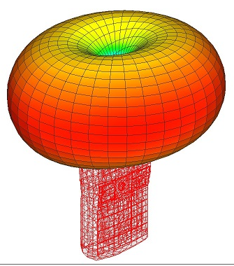
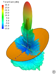
Directivity is a measure of how directional an antenna’s radiation pattern is. For example an antenna that radiates strongly in one direction has a high directivity while an antenna that radiates equally in all directions has a low directivity.

It is not necessarily a bad thing to have an antenna with low directivity, it depends on the application. For example:

To communicate with a geosynchronous satellite 35,786km away we need an antenna that produces a strong beam directed towards the satellite. In this case a parabolic dish antenna is often used because it has a high directivity.

Alternatively a mobile phone needs to be able to connect to a cell tower no matter what orientation the phone is held which means no matter what direction it’s antenna is pointing. In this case an antenna with a low directivity is used so that the antenna can receive/transmit well in any direction.

Calculating Directivity

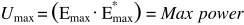
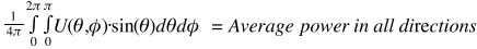
Directivity can be calculated using the equation below which basically means the max value of radiated power divided by the average power in all directions:

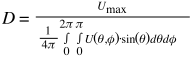
Where:

Directivity is often expressed in dBi and represents the dB ratio with respect to an isotropic radiator.

Python Script – Directivity.py

The gist below shows my Python script for calculating the directivity (based on the ArrayCalc calc_directivity.m file).

The main function is:

CalcDirectivity(Efficiency, RadPatternFunction, *args)

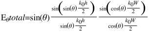
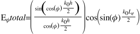
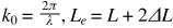
This takes a function argument, RadPatternFunction, as an input. This function should describe the antennas radiation pattern in terms of theta and phi.

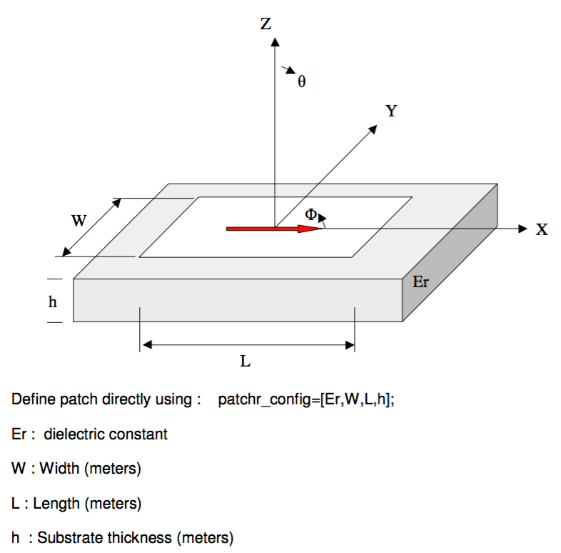
At the bottom of the script there are some basic examples showing how to calculate the directivity for three different radiation patterns – an isotropic antenna and two sin functions. Below this there are also two examples calculating the directivity for rectangular patches using the functions discussed in my Square Patch Element post.

The efficiency argument to RadPatternFunction is related to the Gain of the antenna and will be discussed in my next post.

Antenna Arrays And Python – Square Patch Element

As mentioned in my intro post, the individual antennas in an array are often known as “elements”. To compute the arrays performance each individual elements field contribution needs to be summed. For my initial investigation I focus on using a rectangular microstrip patch element and this post will cover the model that is used.

A microstrip or patch antenna is a low profile antenna that has a number of advantages over other antennas – it is lightweight, inexpensive, and easy to integrate with accompanying electronics because they can be printed directly onto a circuit board which makes them easy to fabricate.

A patch antenna usually consists of a conductive patch with width W, and length L, sitting on top of a substrate (i.e. a dielectric circuit board) with thickness h and relative permittivity Er. The substrate then sits on top of a conductive ground plane.

With the model used there is no account taken of mutual coupling between the elements. This can have a significant effect on array performance when array elements themselves are large, elements are closely spaced or large scan angles are used. It is also assumed the ground plane is infinite so the model is only valid over 0°<theta<90°, 0°<phi < 360°. The benefits of this model are the calculation is potentially very fast and despite the limitations the model still provides enough accuracy to give a useful insight into the potential performance of an array, before committing to more detailed modelling or prototyping.

The E theta and E phi components of the far-field radiation pattern are given by the equations below:

Using these equations allows us to create the following Python function to calculate the total E-field pattern for the patch as a function of theta and phi:

Before moving on to the array calculation itself next time I’ll detail the Python scripts I use to visualise the fields as it’s always nice to see what’s going on.

Blockchains & Digital Currency

Warning, this is a bit of a brain spew!

Digital currency such as Bitcoin and Ethereum and the blockchains they are built on are exciting and interesting technologies. I’ve been following various blogs about them for some time and there are often comparrisons to the early days of the internet. If that’s the case I want to be involved! But I’m not sure of the best way. And is it going to live up to the hype?

There appear to be two obvious ways to get into it. Firstly develop using the technologies or secondly – speculate on the associated currencies/tokens. I don’t know if I have the creativity or the time to dive into the development side of things although I do find it interesting, especially Ethereum. Speculating on the currency is easy enough to do, just purchase some, but it’s really just guess work, think I need to come up with some kind of strategy.