Antenna Arrays And Python – Square Patch Element

As mentioned in my intro post, the individual antennas in an array are often known as “elements”. To compute the arrays performance each individual elements field contribution needs to be summed. For my initial investigation I focus on using a rectangular microstrip patch element and this post will cover the model that is used.
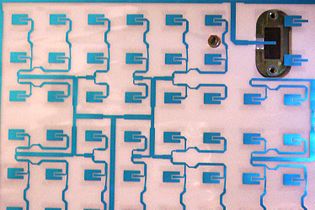
A microstrip or patch antenna is a low ­profile antenna that has a number of advantages over other antennas – it is lightweight, inexpensive, and easy to integrate with accompanying electronics because they can be printed directly onto a circuit board which makes them easy to fabricate.

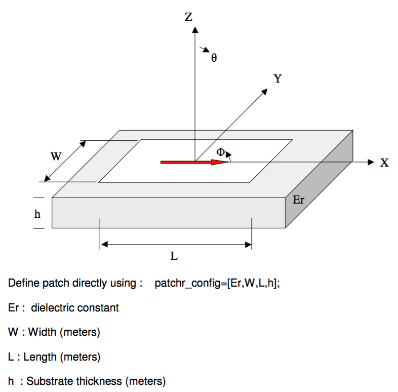
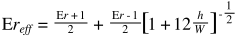
A patch antenna usually consists of a conductive patch with width W, and length L, sitting on top of a substrate (i.e. a dielectric circuit board) with thickness h and relative permittivity Er. The substrate then sits on top of a conductive ground plane.


Patch Antenna (taken from ArrayCalc)
The element model is taken from C.A. Balanis 2nd Edition Page 745, and represents the far-field element radiation patterns as closed form mathematical equations. The model used is the cavity/transmission-line model and is referenced by most antenna texts covering microstrip antennas. The patch is modelled as 2 radiating slots, separated by a nominally half wavelength section of low impedance transmission line. The calculations are fully detailed in the ArrayCalc Design_patchr.m file and also the theory is detailed in the Theory Of Operation document. I also find the antenna-theory website a useful resource for further reading.

With the model used there is no account taken of mutual coupling between the elements. This can have a significant effect on array performance when array elements themselves are large, elements are closely spaced or large scan angles are used. It is also assumed the ground plane is infinite so the model is only valid over 0°<theta<90°, 0°<phi < 360°. The benefits of this model are the calculation is potentially very fast and despite the limitations the model still provides enough accuracy to give a useful insight into the potential performance of an array, before committing to more detailed modelling or prototyping.

The E theta and E phi components of the far-field radiation pattern are given by the equations below:

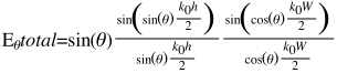
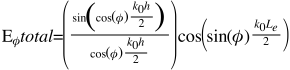
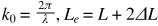
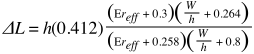
Using these equations allows us to create the following Python function to calculate the total E-field pattern for the patch as a function of theta and phi:

Before moving on to the array calculation itself next time I’ll detail the Python scripts I use to visualise the fields as it’s always nice to see what’s going on.

Antenna Arrays And Python – ArrayCalc & Coordinate Systems

I want to start by acknowledging that the basis for most of the Python scripts came from Neill Tucker’s Antennas and Microwave page and more specifically his Phased Array Design Toolbox called ArrayCalc. He seems to really (really, really) know his antennas and his site has a lot of very useful and interesting theory and practical examples, totally worth checking out.

ArrayCalc is an extremely detailed and powerful toolbox written for Matlab that enables analysis of 2D and 3D antenna arrays with various built in antenna elements available such as dipoles, rectangular and circular microstrip patches and helixes. The code is all provided and the documentation is superb and really helped me understand the theory. The only issue for me is I don’t have access to Matlab! I decided to try and cherry pick the code that could be useful for me and rewrite it in Python.

Coordinate System

In ArrayCalc, Theory of Operation documentation Neill states that in his first antenna design job his mentor advised – “if you want to be a good antenna engineer, get your head around 3D coordinate geometry”. This is sound advice. Once I got it clear in my head the definitions of the spherical and cartesian coordinate systems and how they were related I found processing of the various output graphs, etc easier to understand and had a more intuitive feel for what was going on with the antennas.

The global coordinate system is established as a reference for the antenna array as a whole. It can be defined in both cartesian and spherical coordinates and the transforms between the two are shown in the diagram below. In my scripts an array of elements will be defined along the x-y plane with each element having its own x, y, z position with z always being zero. Neill provides a lot of detail regarding his geometrical set-up in the Theory of Operation documentation which is worth a read for more understanding.

Coordinate Systems

Antenna Arrays And Python – Introduction

I’ve been delving into the world of antenna arrays recently. The thing that really helped me understand the background theory was writing some Python scripts covering some design calculations. I wanted to detail some of these to help finalise my thoughts and to possibly assist anyone looking at this kind of thing.

There’s a lot of theory and terminology around antennas that could make some of the details unclear. If anyones interested and struggling let me know and I’ll do my best to help or at least point you in the right direction of further reading.

Antenna Array Overview

As a very simple overview an antenna array is a set of individual antennas which are connected together. Basically, it’s possible to design an array to be more sensitive in the desired direction than the individual antennas would be by themselves. When designed correctly the radio waves radiated by each individual antenna combine, adding together to enhance the power radiated in desired directions, and cancelling to reduce the power radiated in other directions. Due to reciprocity the same will also happen with radio waves being received.

Another useful function of array antennas can be electronic beam scanning. By phasing each antenna separately the beam of radio waves can be steered electronically to point instantly in any direction over a wide angle. This is most often referred to as a “phased array”.

Antenna Elements

The individual antennas in an array are often known as “elements”. The elements considered in most literature are microstrip patches but in theory an element can be any radiating antenna such as the dishes shown in the picture below.

Microstrip array, made up of 38 patch antennas
Very Large Array, made up of 27 dish antennas

In my next post I plan to cover the work done on a rectangular microstrip patch design that will then go on to function as an element in an array.

Deploying a Django app to Heroku

Note to self — before deploying a local Django app to Heroku I should do the following:

Install the wsgi HTTP server, gunicorn:

pip install gunicorn

Install package to help work with environment variables:

pip install python-dotenv

Install Python-PostgreSQL Database Adapter:

pip install psycopg2

Create requirements file:

pip freeze > requirements.txt

Configure settings.py to load environment variables and the database:

import dotenv
import dj_database_url

# this line is already in your settings.py
BASE_DIR = os.path.dirname(os.path.dirname(os.path.abspath(__file__)))

# load environment variables from .env
dotenv_file = os.path.join(BASE_DIR, ".env")
if os.path.isfile(dotenv_file):
    dotenv.load_dotenv(dotenv_file)

# load database from the DATABASE_URL environment variable
DATABASES = {}
DATABASES['default'] = dj_database_url.config(conn_max_age=600)

Also delete the default database config:

DATABASES = {
    'default': {
        'ENGINE': 'django.db.backends.sqlite3',
        'NAME': os.path.join(BASE_DIR, 'db.sqlite3'),
    }
}

Add a .env file to project base directory and add the database URL:

DATABASE_URL=sqlite:///db.sqlite3

Make sure .env is added to .gitignore so it doesn’t get pushed to repo. My last .gitignore looked like:

*.pyc
*~
__pycache__
myvenv
venv
db.sqlite3
.DS_Store
.env

Assuming there is already a heroku account run:

heroku login

locally to associate machine with heroku account.

On the heroku dashboard create a new app. Under the “Settings” tab and under “Buildpacks” add a new buildpack called “heroku/python”.

Under “Config Variables” add “DISABLE_COLLECTSTATIC” with a value of “1”.

To set-up the database go back to command line and enter:

heroku addons:create heroku-postgresql:hobby-dev -a YOUR_APP_NAME

This provisions a new postgres database and should add the url to the Config Variables. Run command:

heroku config -a YOUR_APP_NAME

DATABASE_URL should be added to Config Variables.

Now create a new file called Procfile in the base directory of project and add:

web: gunicorn YOURSITE.wsgi --log-level=info --log-file -

Where YOURSITE is specific to the project.

Add another file in base directory called runtime.txt and add the version of python you want to use:

python-3.5.2

To serve static assets I use the WhiteNoise project. To install:

pip install whitenoise
...
pip freeze > requirements.txt

Add it to the app by changing wsgi.py to include:

from django.core.wsgi import get_wsgi_application
from whitenoise.django import DjangoWhiteNoise

application = get_wsgi_application()
application = DjangoWhiteNoise(application)

Now that should be it! Commit the changes locally then run:

git push heroku master

It should display the progress of installation and eventually be up and running.

References

This was trying to put a bunch of stuff I read in the articles below into an order I’ve found works for me.

https://blog.heroku.com/in_deep_with_django_channels_the_future_of_real_time_apps_in_django