I want to start by acknowledging that the basis for most of the Python scripts came from Neill Tucker’s Antennas and Microwave page and more specifically his Phased Array Design Toolbox called ArrayCalc. He seems to really (really, really) know his antennas and his site has a lot of very useful and interesting theory and practical examples, totally worth checking out.
ArrayCalc is an extremely detailed and powerful toolbox written for Matlab that enables analysis of 2D and 3D antenna arrays with various built in antenna elements available such as dipoles, rectangular and circular microstrip patches and helixes. The code is all provided and the documentation is superb and really helped me understand the theory. The only issue for me is I don’t have access to Matlab! I decided to try and cherry pick the code that could be useful for me and rewrite it in Python.
Coordinate System
In ArrayCalc, Theory of Operation documentation Neill states that in his first antenna design job his mentor advised – “if you want to be a good antenna engineer, get your head around 3D coordinate geometry”. This is sound advice. Once I got it clear in my head the definitions of the spherical and cartesian coordinate systems and how they were related I found processing of the various output graphs, etc easier to understand and had a more intuitive feel for what was going on with the antennas.
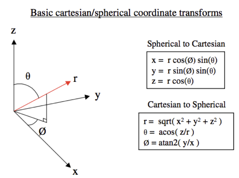
The global coordinate system is established as a reference for the antenna array as a whole. It can be defined in both cartesian and spherical coordinates and the transforms between the two are shown in the diagram below. In my scripts an array of elements will be defined along the x-y plane with each element having its own x, y, z position with z always being zero. Neill provides a lot of detail regarding his geometrical set-up in the Theory of Operation documentation which is worth a read for more understanding.
