One of the most useful things to see when investigating an antenna design is the radiation pattern – a plot showing where the antenna transmits or receives power. In the previous post a Python function was developed for a square patch that calculated the total E-field pattern as a function of theta and phi. Now I want to plot this E-field which will show the radiation pattern.
matplotlib
I don’t have a great deal of experience with visualisation or plotting in Python but I have used matplotlib before and found it relatively ok. matplotlib is a plotting library for the Python programming language and Pyplot is a matplotlib module that provides a collection of command style functions to make matplotlib work like MATLAB.
This Pyplot tutorial covers the basics and I find the gallery useful to find example code.
E-plane & H-plane plots
First plots I wanted to see were for E-field vs 0°<theta<90 °for phi cuts at 0° and 90°. Referring to the patch geometry we described earlier this will give us the E-plane (phi = 0°) and the H-plane (phi = 90°).

An example plot of a patch with W=7mm, L=5.58mm, Er=3.66, h=10.1mm is shown below. The complete Python script can be found at the end of the post with the relevant function being: PatchEHPlanePlot(freq, W, L, h, Er).

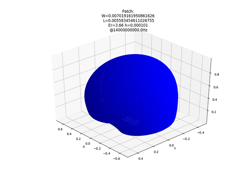
3d surface plot
The next plot I wanted was a 3D plot of the E-field across all phi and theta values. This will allow the visualisation of things like the main beam direction, side lobes, etc. While it is nice to see this for the patch it will be very helpful when it comes to investigating a full array.
An example of the surface plot for the same rectangular microstrip element is shown below and was plotted using the SurfacePlot(Fields) function in the code.
Patch Script
The completed patch script can be seen below. It consists of the following functions:
main: Some examples of various patch designs.
DesignPatch(Er, h, Freq): Theory taken from ArrayCalc. It returns the patch L & W for specified Er, h and freq.
SurfacePlot(Fields, Freq, W, L, h, Er): Plots a 3D surface of the field.
PatchEHPlanePlot(Freq, W, L, h, Er, isLog=True): Plots the 2D E&H-planes.
GetPatchFields(PhiStart, PhiStop, ThetaStart, ThetaStop, Freq, W, L, h, Er): Returns an array with fields for patch over phi and theta range.
PatchFunction(thetaInDeg, phiInDeg, Freq, W, L, h, Er): Calculates total E-field pattern for patch as a function of theta and phi as detailed in previous post.