Recently I’ve been using Python and Cartopy to plot some Latitude/Longitude data on a map. Initially it took some time to figure out how to get it to work so I thought I’d share my code incase it was useful.
According to the Cartopy intro it is
“a Python package designed to make drawing maps for data analysis and visualisation as easy as possible.”
I’m not sure how active the project is and I found the documentation a bit lacking but once I was up and running it was pretty easy to use and I think the results look pretty good.
Plotting My Data
I have a csv file with various data timestamped and saved on each line. For this case I was interested in the lat/lng location, signal strength (for an antenna) and also a satellite number. An example of one line of data is:
2017–07–10 22:31:59:203,Processing UpdatePacket: [‘:’, ‘1’, ‘0’, ‘0’, ‘1’, ‘0’, ‘0’, ‘1.63’, ‘17.15’, ‘246.57’, ‘114.11’, ‘57.008263’, ‘-5.827861’, ‘310.00’, ‘1’, ‘NAN’, ‘0’, ‘2’, ‘0’, ‘c\n’]
and from that the information I require is:
lat/lng position: 57.008263,-5.827861
signal strength: 1.63
satellite number: 310.00
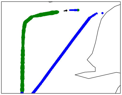
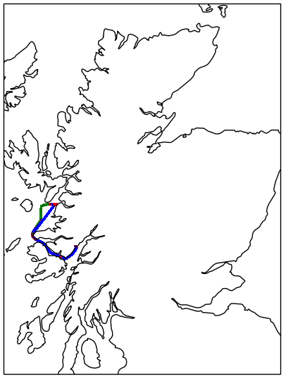
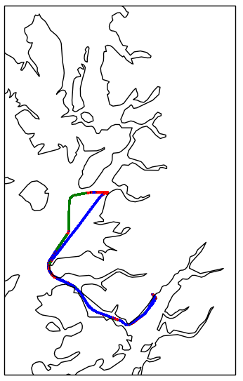
Initially for each lat/lng position I wanted to plot the point on a map and colour the marker at that point to show which satellite number it was. Also if the signal strength was -100 the marker colour should be shown as red. An example taken from some of the data is shown below.
The following Gist shows the Python script I used:
Script Details
Most of the script is actually concerned with reading the file and parsing the relevant data. The main plotting functionality is in the section:
ax = plt.axes(projection=ccrs.Mercator()) # Map projection
ax.coastlines(resolution=’10m’)           # Adds coastline to map at highest resolution

plt.scatter(lngArr, latArr, s=area, c=satLngArr, alpha=0.5, transform=ccrs.Geodetic())                # Plot
plt.show()
The projection sets the coordinate system and is selected from the Cartopy projection list (there’s a lot to pick from and I chose the one I thought looked the best).
Next a coastline is added to the projection. As I was focusing on a small section of Scottish coastline I went with the 10m resolution which is the highest but lower resolutions can be selected as detailed in the documentation.
Finally a scatter plot is created. The data has been parsed into equal sized lists of longitude and latitude points.
The ‘s’ parameter defines the size of the marker at each point, in this case all set to 1pt radii.
The ‘c’ parameter defines the colour of the marker, in this case blue for satellite 310, green for 60, yellow for 302, black for any other satellite and red if signal strength is -100.
Finally the transform=ccrs.Geodetic() sets the lat/lng coordinate system as defined here.
Scaling Marker Size
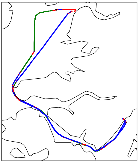
It’s also possible to adjust the radius of the marker at each point. To scale it relative to the signal strength (I removed the -100 strengths):
area = np.pi * (strengthNpArray)**2
Which gives: