Antenna Arrays And Python – The Array (finally!)

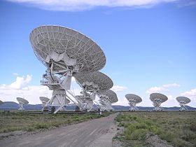
As mentioned in my intro post an array antenna is a set of individual antennas connected to work as a single antenna. So far we’ve covered the individual antennas, i.e. the square patches, now it’s time to look at how they can be connected to work together.

Array Factor Fun

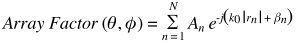
You can’t get far digging into arrays before you come across the Array Factor. It looks complicated but to me the easiest way to think of it is that it combines every elements position, radiating amplitude and radiating phase to give the overall array performance.

The Array Factor demonstrates that by altering an element, such as its position or phase, we can alter the arrays properties. For example the arrays beam could be steered to a desired position by altering the phase of each element.

The Array Factor is given by:

Where:

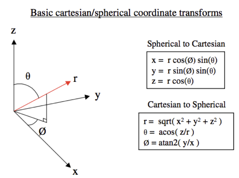
θ, φ = Direction from origin

N = number of elements

An= Amp of element

βn = Phase of element in rads

k0 = 2π/λ rads/m

And:

is the relative phase of incident wave at element n located at xn, yn, zn.

Array Factor in Python

The script below shows how easy it is to calculate the Array Factor in Python:

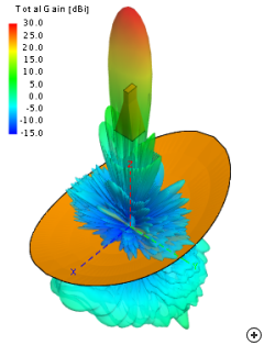
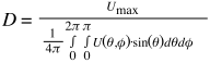
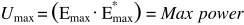
Array Radiation Pattern, Directivity & Gain

The above Array Factor equation is independent of each elements individual radiating pattern. The overall radiation pattern of an array is determined by the array factor combined with the radiation pattern of each element, Fn(θn, φn), giving:

The overall radiation pattern results in a certain directivity and thus gain linked through the efficiency as discussed previously.

Some Examples

To demonstrate the effects the individual element patterns have on the overall array performance we can investigate some examples using Python.

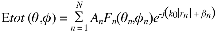
Isotropic antenna elements

In this case each element radiates equally in all directions so Fn(θn, φn) is the same for each θn, φn. The antenna radiation pattern is now just the Array Factor as described in the code above.

15×15 Array of Isotropic Elements

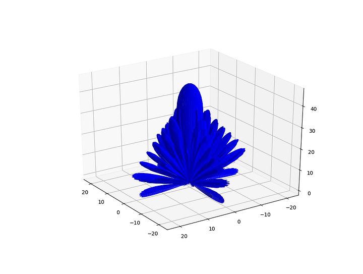
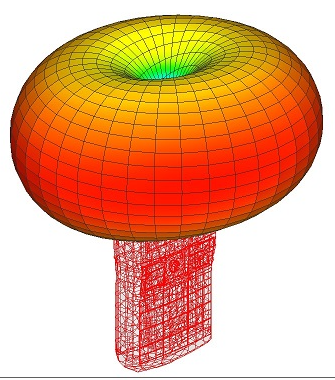
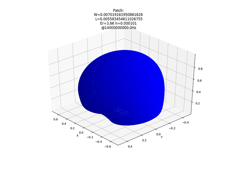
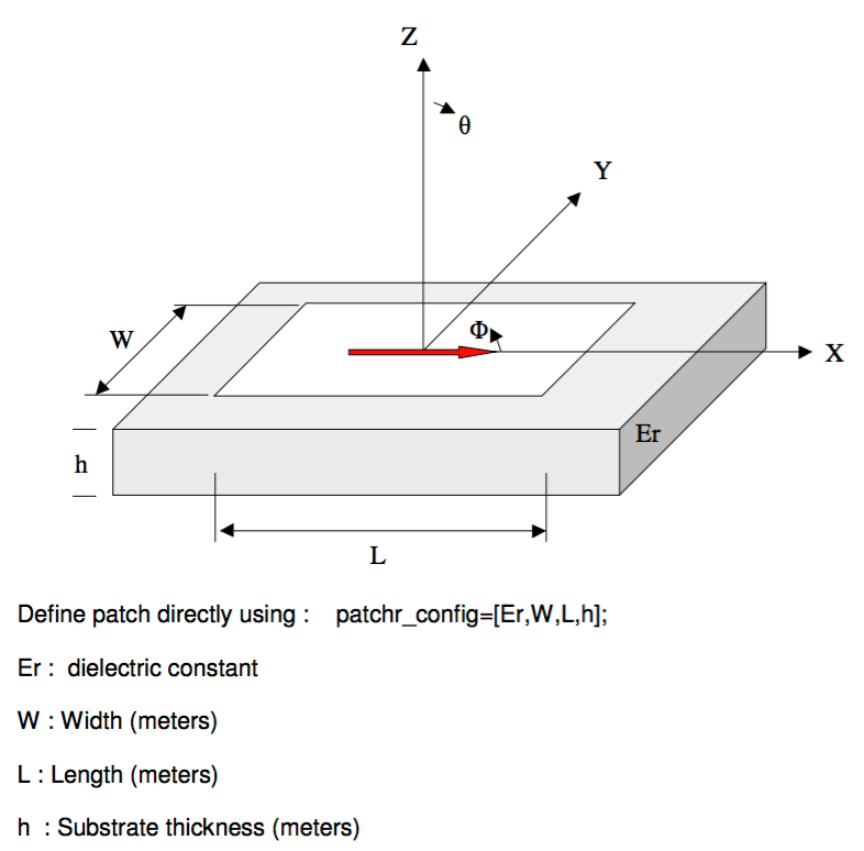
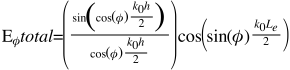
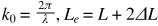
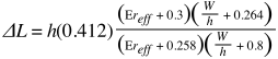
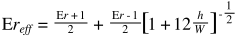
Patch antenna elements

Using elements described by the PatchFunction discussed previously:

PatchFunction(θ, φ, Freq, 10.7e-3, 10.47e-3, 3e-3, 2.5)
15×15 Array of patches

Python script for patch array:

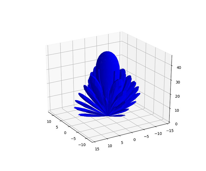
Horn antenna elements

And finally using horn antenna elements represented by cos²⁸(θ) function.

15×15 Array of cos²⁸(θ) Horns

Python script for horn array:

Next time we can see how to calculate an elements phase to steer the beam.

Antenna Arrays And Python – Patch Efficiency & Gain

Last post I dealt with antenna directivity, this post discusses antenna gain which is closely related.

Gain combines an antennas directivity and efficiency to describe how good it is at sending/receiving power in a direction. This is useful for things like link budget analysis which basically calculates if two antennas can communicate.

Antenna Gain, G, can be calculate from the directivity, D, and antenna efficiency, εr by:

The efficiency of an antenna describes how well the input power is radiated by the antenna (and due to reciprocity receive efficiency is the same as transmit efficiency):

A high efficiency antenna will radiate most of the input power while a low efficiency antenna will lose a lot of the input power before it is radiated due to things like dielectric loss, impedance mismatch, etc.

Patch Efficiency

The Python script at the bottom of the post is based on the ArrayCalc calc_patchr_eff.m file and defines a function, CalculatePatchEff, that calculate the efficiency of a rectangular patch based on the patch dimensions and materials. The comments provide some example material properties and the main function has some examples that demonstrate the effects of the material selection on the efficiency:

FR4 Patch, 14GHz, Efficiency = 47.27%

RO4350 Patch, 14GHz, Efficiency = 62.32%

Python Script

Antenna Arrays And Python – Calculating Directivity

Directivity is a measure of how directional an antenna’s radiation pattern is. For example an antenna that radiates strongly in one direction has a high directivity while an antenna that radiates equally in all directions has a low directivity.

It is not necessarily a bad thing to have an antenna with low directivity, it depends on the application. For example:

To communicate with a geosynchronous satellite 35,786km away we need an antenna that produces a strong beam directed towards the satellite. In this case a parabolic dish antenna is often used because it has a high directivity.

Alternatively a mobile phone needs to be able to connect to a cell tower no matter what orientation the phone is held which means no matter what direction it’s antenna is pointing. In this case an antenna with a low directivity is used so that the antenna can receive/transmit well in any direction.


Mobile Phone Pattern — Low Directivity


Dish Pattern — High Directivity

Calculating Directivity

Directivity can be calculated using the equation below which basically means the max value of radiated power divided by the average power in all directions:

Where:

Directivity is often expressed in dBi and represents the dB ratio with respect to an isotropic radiator.

Python Script – Directivity.py

The gist below shows my Python script for calculating the directivity (based on the ArrayCalc calc_directivity.m file).

The main function is:

CalcDirectivity(Efficiency, RadPatternFunction, *args)

This takes a function argument, RadPatternFunction, as an input. This function should describe the antennas radiation pattern in terms of theta and phi.

At the bottom of the script there are some basic examples showing how to calculate the directivity for three different radiation patterns – an isotropic antenna and two sin functions. Below this there are also two examples calculating the directivity for rectangular patches using the functions discussed in my Square Patch Element post.

The efficiency argument to RadPatternFunction is related to the Gain of the antenna and will be discussed in my next post.

Antenna Arrays And Python – Plotting with Pyplot

One of the most useful things to see when investigating an antenna design is the radiation pattern – a plot showing where the antenna transmits or receives power. In the previous post a Python function was developed for a square patch that calculated the total E-field pattern as a function of theta and phi. Now I want to plot this E-field which will show the radiation pattern.

matplotlib

I don’t have a great deal of experience with visualisation or plotting in Python but I have used matplotlib before and found it relatively ok. matplotlib is a plotting library for the Python programming language and Pyplot is a matplotlib module that provides a collection of command style functions to make matplotlib work like MATLAB.

This Pyplot tutorial covers the basics and I find the gallery useful to find example code.

E-plane & H-plane plots

First plots I wanted to see were for E-field vs 0°<theta<90 °for phi cuts at 0° and 90°. Referring to the patch geometry we described earlier this will give us the E-plane (phi = 0°) and the H-plane (phi = 90°).

Patch geometry

An example plot of a patch with W=7mm, L=5.58mm, Er=3.66, h=10.1mm is shown below. The complete Python script can be found at the end of the post with the relevant function being: PatchEHPlanePlot(freq, W, L, h, Er).

Example E&H-Plane plot

3d surface plot

The next plot I wanted was a 3D plot of the E-field across all phi and theta values. This will allow the visualisation of things like the main beam direction, side lobes, etc. While it is nice to see this for the patch it will be very helpful when it comes to investigating a full array.

An example of the surface plot for the same rectangular microstrip element is shown below and was plotted using the SurfacePlot(Fields) function in the code.

Patch Surface Plot

Patch Script

The completed patch script can be seen below. It consists of the following functions:

main: Some examples of various patch designs.

DesignPatch(Er, h, Freq): Theory taken from ArrayCalc. It returns the patch L & W for specified Er, h and freq.

SurfacePlot(Fields, Freq, W, L, h, Er): Plots a 3D surface of the field.

PatchEHPlanePlot(Freq, W, L, h, Er, isLog=True): Plots the 2D E&H-planes.

GetPatchFields(PhiStart, PhiStop, ThetaStart, ThetaStop, Freq, W, L, h, Er): Returns an array with fields for patch over phi and theta range.

PatchFunction(thetaInDeg, phiInDeg, Freq, W, L, h, Er): Calculates total E-field pattern for patch as a function of theta and phi as detailed in previous post.

Antenna Arrays And Python – Square Patch Element

As mentioned in my intro post, the individual antennas in an array are often known as “elements”. To compute the arrays performance each individual elements field contribution needs to be summed. For my initial investigation I focus on using a rectangular microstrip patch element and this post will cover the model that is used.

A microstrip or patch antenna is a low ­profile antenna that has a number of advantages over other antennas – it is lightweight, inexpensive, and easy to integrate with accompanying electronics because they can be printed directly onto a circuit board which makes them easy to fabricate.

A patch antenna usually consists of a conductive patch with width W, and length L, sitting on top of a substrate (i.e. a dielectric circuit board) with thickness h and relative permittivity Er. The substrate then sits on top of a conductive ground plane.


Patch Antenna (taken from ArrayCalc)
The element model is taken from C.A. Balanis 2nd Edition Page 745, and represents the far-field element radiation patterns as closed form mathematical equations. The model used is the cavity/transmission-line model and is referenced by most antenna texts covering microstrip antennas. The patch is modelled as 2 radiating slots, separated by a nominally half wavelength section of low impedance transmission line. The calculations are fully detailed in the ArrayCalc Design_patchr.m file and also the theory is detailed in the Theory Of Operation document. I also find the antenna-theory website a useful resource for further reading.

With the model used there is no account taken of mutual coupling between the elements. This can have a significant effect on array performance when array elements themselves are large, elements are closely spaced or large scan angles are used. It is also assumed the ground plane is infinite so the model is only valid over 0°<theta<90°, 0°<phi < 360°. The benefits of this model are the calculation is potentially very fast and despite the limitations the model still provides enough accuracy to give a useful insight into the potential performance of an array, before committing to more detailed modelling or prototyping.

The E theta and E phi components of the far-field radiation pattern are given by the equations below:

Using these equations allows us to create the following Python function to calculate the total E-field pattern for the patch as a function of theta and phi:

Before moving on to the array calculation itself next time I’ll detail the Python scripts I use to visualise the fields as it’s always nice to see what’s going on.

Antenna Arrays And Python – ArrayCalc & Coordinate Systems

I want to start by acknowledging that the basis for most of the Python scripts came from Neill Tucker’s Antennas and Microwave page and more specifically his Phased Array Design Toolbox called ArrayCalc. He seems to really (really, really) know his antennas and his site has a lot of very useful and interesting theory and practical examples, totally worth checking out.

ArrayCalc is an extremely detailed and powerful toolbox written for Matlab that enables analysis of 2D and 3D antenna arrays with various built in antenna elements available such as dipoles, rectangular and circular microstrip patches and helixes. The code is all provided and the documentation is superb and really helped me understand the theory. The only issue for me is I don’t have access to Matlab! I decided to try and cherry pick the code that could be useful for me and rewrite it in Python.

Coordinate System

In ArrayCalc, Theory of Operation documentation Neill states that in his first antenna design job his mentor advised – “if you want to be a good antenna engineer, get your head around 3D coordinate geometry”. This is sound advice. Once I got it clear in my head the definitions of the spherical and cartesian coordinate systems and how they were related I found processing of the various output graphs, etc easier to understand and had a more intuitive feel for what was going on with the antennas.

The global coordinate system is established as a reference for the antenna array as a whole. It can be defined in both cartesian and spherical coordinates and the transforms between the two are shown in the diagram below. In my scripts an array of elements will be defined along the x-y plane with each element having its own x, y, z position with z always being zero. Neill provides a lot of detail regarding his geometrical set-up in the Theory of Operation documentation which is worth a read for more understanding.

Coordinate Systems

Antenna Arrays And Python – Introduction

I’ve been delving into the world of antenna arrays recently. The thing that really helped me understand the background theory was writing some Python scripts covering some design calculations. I wanted to detail some of these to help finalise my thoughts and to possibly assist anyone looking at this kind of thing.

There’s a lot of theory and terminology around antennas that could make some of the details unclear. If anyones interested and struggling let me know and I’ll do my best to help or at least point you in the right direction of further reading.

Antenna Array Overview

As a very simple overview an antenna array is a set of individual antennas which are connected together. Basically, it’s possible to design an array to be more sensitive in the desired direction than the individual antennas would be by themselves. When designed correctly the radio waves radiated by each individual antenna combine, adding together to enhance the power radiated in desired directions, and cancelling to reduce the power radiated in other directions. Due to reciprocity the same will also happen with radio waves being received.

Another useful function of array antennas can be electronic beam scanning. By phasing each antenna separately the beam of radio waves can be steered electronically to point instantly in any direction over a wide angle. This is most often referred to as a “phased array”.

Antenna Elements

The individual antennas in an array are often known as “elements”. The elements considered in most literature are microstrip patches but in theory an element can be any radiating antenna such as the dishes shown in the picture below.

Microstrip array, made up of 38 patch antennas
Very Large Array, made up of 27 dish antennas

In my next post I plan to cover the work done on a rectangular microstrip patch design that will then go on to function as an element in an array.